How Google Finds Your Needle in the Web's Haystack
As we'll see, the trick is to ask the web itself to rank the importance of pages...
Imagine a library containing 25 billion documents but with no centralized organization and no librarians. In addition, anyone may add a document at any time without telling anyone. You may feel sure that one of the documents contained in the collection has a piece of information that is vitally important to you, and, being impatient like most of us, you'd like to find it in a matter of seconds. How would you go about doing it?
Posed in this way, the problem seems impossible. Yet this description is not too different from the World Wide Web, a huge, highly-disorganized collection of documents in many different formats. Of course, we're all familiar with search engines (perhaps you found this article using one) so we know that there is a solution. This article will describe Google's PageRank algorithm and how it returns pages from the web's collection of 25 billion documents that match search criteria so well that "google" has become a widely used verb.
Most search engines, including Google, continually run an army of computer programs that retrieve pages from the web, index the words in each document, and store this information in an efficient format. Each time a user asks for a web search using a search phrase, such as "search engine," the search engine determines all the pages on the web that contains the words in the search phrase. (Perhaps additional information such as the distance between the words "search" and "engine" will be noted as well.) Here is the problem: Google now claims to index 25 billion pages. Roughly 95% of the text in web pages is composed from a mere 10,000 words. This means that, for most searches, there will be a huge number of pages containing the words in the search phrase. What is needed is a means of ranking the importance of the pages that fit the search criteria so that the pages can be sorted with the most important pages at the top of the list.
One way to determine the importance of pages is to use a human-generated ranking. For instance, you may have seen pages that consist mainly of a large number of links to other resources in a particular area of interest. Assuming the person maintaining this page is reliable, the pages referenced are likely to be useful. Of course, the list may quickly fall out of date, and the person maintaining the list may miss some important pages, either unintentionally or as a result of an unstated bias.
Google's PageRank algorithm assesses the importance of web pages without human evaluation of the content. In fact, Google feels that the value of its service is largely in its ability to provide unbiased results to search queries; Google claims, "the heart of our software is PageRank." As we'll see, the trick is to ask the web itself to rank the importance of pages.
How to tell who's important
If you've ever created a web page, you've probably included links to other pages that contain valuable, reliable information. By doing so, you are affirming the importance of the pages you link to. Google's PageRank algorithm stages a monthly popularity contest among all pages on the web to decide which pages are most important. The fundamental idea put forth by PageRank's creators, Sergey Brin and Lawrence Page, is this: the importance of a page is judged by the number of pages linking to it as well as their importance.
We will assign to each web page P a measure of its importance I(P), called the page's PageRank. At various sites, you may find an approximation of a page's PageRank. (For instance, the home page of The American Mathematical Society currently has a PageRank of 8 on a scale of 10. Can you find any pages with a PageRank of 10?) This reported value is only an approximation since Google declines to publish actual PageRanks in an effort to frustrate those would manipulate the rankings.
Here's how the PageRank is determined. Suppose that page Pj has lj links. If one of those links is to page Pi, then Pj will pass on 1/lj of its importance to Pi. The importance ranking of Pi is then the sum of all the contributions made by pages linking to it. That is, if we denote the set of pages linking to Pi by Bi, then
![\[ I(P_i)=\sum_{P_j\in B_i} \frac{I(P_j)}{l_j} \]](http://www.ams.org/featurecolumn/images/december2006/index_1.gif)
This may remind you of the chicken and the egg: to determine the importance of a page, we first need to know the importance of all the pages linking to it. However, we may recast the problem into one that is more mathematically familiar.
Let's first create a matrix, called the hyperlink matrix, ![$ {\bf H}=[H_{ij}] $](http://www.ams.org/featurecolumn/images/december2006/index_2.gif) in which the entry in the ith row and jth column is
![\[ H_{ij}=\left\{\begin{array}{ll}1/l_{j} & \hbox{if } P_j\in B_i \\ 0 & \hbox{otherwise} \end{array}\right. \]](http://www.ams.org/featurecolumn/images/december2006/index_3.gif)
Notice that H has some special properties. First, its entries are all nonnegative. Also, the sum of the entries in a column is one unless the page corresponding to that column has no links. Matrices in which all the entries are nonnegative and the sum of the entries in every column is one are called stochastic; they will play an important role in our story.
We will also form a vector ![$ I=[I(P_i)] $](http://www.ams.org/featurecolumn/images/december2006/index_4.gif) whose components are PageRanks--that is, the importance rankings--of all the pages. The condition above defining the PageRank may be expressed as
![\[ I = {\bf H}I \]](http://www.ams.org/featurecolumn/images/december2006/index_5.gif)
In other words, the vector I is an eigenvector of the matrix H with eigenvalue 1. We also call this a stationary vector of H.
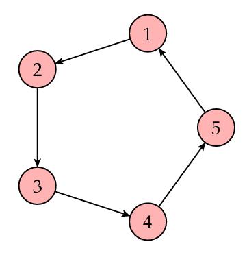
Let's look at an example. Shown below is a representation of a small collection (eight) of web pages with links represented by arrows.
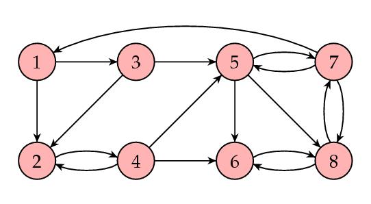
The corresponding matrix is
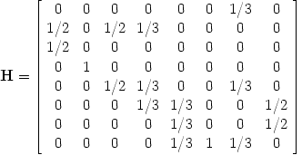 |
with stationary vector
| 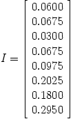 |
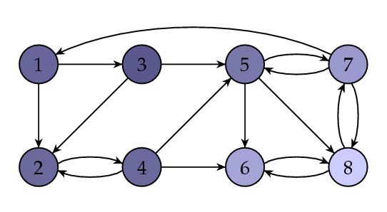
This shows that page 8 wins the popularity contest. Here is the same figure with the web pages shaded in such a way that the pages with higher PageRanks are lighter.
Computing I
There are many ways to find the eigenvectors of a square matrix. However, we are in for a special challenge since the matrix H is a square matrix with one column for each web page indexed by Google. This means that H has about n = 25 billion columns and rows. However, most of the entries in H are zero; in fact, studies show that web pages have an average of about 10 links, meaning that, on average, all but 10 entries in every column are zero. We will choose a method known as the power method for finding the stationary vector I of the matrix H.
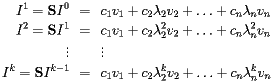
How does the power method work? We begin by choosing a vector I 0 as a candidate for I and then producing a sequence of vectors I k by
![\[ I^{k+1}={\bf H}I^k \]](http://www.ams.org/featurecolumn/images/december2006/index_6.gif)
The method is founded on the following general principle that we will soon investigate.
General principle: The sequence I k will converge to the stationary vector I.
|
We will illustrate with the example above.
| I 0 | I 1 | I 2 | I 3 | I 4 | ... | I 60 | I 61 |
| 1 | 0 | 0 | 0 | 0.0278 | ... | 0.06 | 0.06 |
| 0 | 0.5 | 0.25 | 0.1667 | 0.0833 | ... | 0.0675 | 0.0675 |
| 0 | 0.5 | 0 | 0 | 0 | ... | 0.03 | 0.03 |
| 0 | 0 | 0.5 | 0.25 | 0.1667 | ... | 0.0675 | 0.0675 |
| 0 | 0 | 0.25 | 0.1667 | 0.1111 | ... | 0.0975 | 0.0975 |
| 0 | 0 | 0 | 0.25 | 0.1806 | ... | 0.2025 | 0.2025 |
| 0 | 0 | 0 | 0.0833 | 0.0972 | ... | 0.18 | 0.18 |
| 0 | 0 | 0 | 0.0833 | 0.3333 | ... | 0.295 | 0.295 |
It is natural to ask what these numbers mean. Of course, there can be no absolute measure of a page's importance, only relative measures for comparing the importance of two pages through statements such as "Page A is twice as important as Page B." For this reason, we may multiply all the importance rankings by some fixed quantity without affecting the information they tell us. In this way, we will always assume, for reasons to be explained shortly, that the sum of all the popularities is one.
Three important questions
Three questions naturally come to mind:
- Does the sequence I k always converge?
- Is the vector to which it converges independent of the initial vector I 0?
- Do the importance rankings contain the information that we want?
Given the current method, the answer to all three questions is "No!" However, we'll see how to modify our method so that we can answer "yes" to all three.
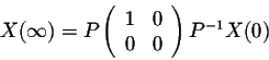
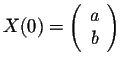
Let's first look at a very simple example. Consider the following small web consisting of two web pages, one of which links to the other:
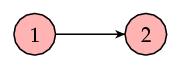 |
with matrix
| 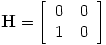 |
Here is one way in which our algorithm could proceed:
In this case, the importance rating of both pages is zero, which tells us nothing about the relative importance of these pages. The problem is that P2 has no links. Consequently, it takes some of the importance from page P1 in each iterative step but does not pass it on to any other page. This has the effect of draining all the importance from the web. Pages with no links are called dangling nodes, and there are, of course, many of them in the real web we want to study. We'll see how to deal with them in a minute, but first let's consider a new way of thinking about the matrix H and stationary vector I.
A probabilitistic interpretation of H
Imagine that we surf the web at random; that is, when we find ourselves on a web page, we randomly follow one of its links to another page after one second. For instance, if we are on page Pj with lj links, one of which takes us to page Pi, the probability that we next end up on Pipage is then  .
As we surf randomly, we will denote by  the fraction of time that we spend on page Pj. Then the fraction of the time that we end up on page Pi page coming from Pj is  . If we end up on Pi, we must have come from a page linking to it. This means that
![\[ T_i = \sum_{P_j\in B_i} T_j/l_j \]](http://www.ams.org/featurecolumn/images/december2006/index_10.gif)
where the sum is over all the pages Pj linking to Pi. Notice that this is the same equation defining the PageRank rankings and so  . This allows us to interpret a web page's PageRank as the fraction of time that a random surfer spends on that web page. This may make sense if you have ever surfed around for information about a topic you were unfamiliar with: if you follow links for a while, you find yourself coming back to some pages more often than others. Just as "All roads lead to Rome," these are typically more important pages.
Notice that, given this interpretation, it is natural to require that the sum of the entries in the PageRank vector I be one.
Of course, there is a complication in this description: If we surf randomly, at some point we will surely get stuck at a dangling node, a page with no links. To keep going, we will choose the next page at random; that is, we pretend that a dangling node has a link to every other page. This has the effect of modifying the hyperlink matrix H by replacing the column of zeroes corresponding to a dangling node with a column in which each entry is 1/n. We call this new matrix S.
In our previous example, we now have
|
with matrix
| 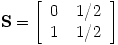 |
and eigenvector
|  |
In other words, page P2 has twice the importance of page P1, which may feel about right to you.
The matrix S has the pleasant property that the entries are nonnegative and the sum of the entries in each column is one. In other words, it is stochastic. Stochastic matrices have several properties that will prove useful to us. For instance, stochastic matrices always have stationary vectors.
For later purposes, we will note that S is obtained from H in a simple way. If A is the matrix whose entries are all zero except for the columns corresponding to dangling nodes, in which each entry is 1/n, then S = H + A.
How does the power method work?
In general, the power method is a technique for finding an eigenvector of a square matrix corresponding to the eigenvalue with the largest magnitude. In our case, we are looking for an eigenvector of S corresponding to the eigenvalue 1. Under the best of circumstances, to be described soon, the other eigenvalues of S will have a magnitude smaller than one; that is,  if  is an eigenvalue of S other than 1.
We will assume that the eigenvalues of S are  and that
![\[ 1 = \lambda_1 > |\lambda_2| \geq |\lambda_3| \geq \ldots \geq |\lambda_n| \]](http://www.ams.org/featurecolumn/images/december2006/index_15.gif)
We will also assume that there is a basis vj of eigenvectors for S with corresponding eigenvalues  . This assumption is not necessarily true, but with it we may more easily illustrate how the power method works. We may write our initial vector I 0 as
![\[ I^0 = c_1v_1+c_2v_2 + \ldots + c_nv_n \]](http://www.ams.org/featurecolumn/images/december2006/index_17.gif)
Then
Since the eigenvalues  with  have magnitude smaller than one, it follows that  if  and therefore  , an eigenvector corresponding to the eigenvalue 1.
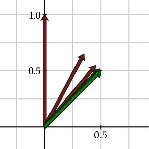
It is important to note here that the rate at which  is determined by  . When  is relatively close to 0, then  relatively quickly. For instance, consider the matrix
![\[ {\bf S} = \left[\begin{array}{cc}0.65 & 0.35 \\ 0.35 & 0.65 \end{array}\right]. \]](http://www.ams.org/featurecolumn/images/december2006/index_28.gif)
The eigenvalues of this matrix are  and  . In the figure below, we see the vectors I k, shown in red, converging to the stationary vector I shown in green.
Now consider the matrix
![\[ {\bf S} = \left[\begin{array}{cc}0.85 & 0.15 \\ 0.15 & 0.85 \end{array}\right]. \]](http://www.ams.org/featurecolumn/images/december2006/index_31.gif)
Here the eigenvalues are  and  . Notice how the vectors I k converge more slowly to the stationary vector I in this example in which the second eigenvalue has a larger magnitude.

When things go wrong
In our discussion above, we assumed that the matrix S had the property that  and  . This does not always happen, however, for the matrices S that we might find.
Suppose that our web looks like this:
In this case, the matrix S is
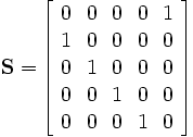
Then we see
| I 0 | I 1 | I 2 | I 3 | I 4 | I 5 |
| 1 | 0 | 0 | 0 | 0 | 1 |
| 0 | 1 | 0 | 0 | 0 | 0 |
| 0 | 0 | 1 | 0 | 0 | 0 |
| 0 | 0 | 0 | 1 | 0 | 0 |
| 0 | 0 | 0 | 0 | 1 | 0 |
In this case, the sequence of vectors I k fails to converge. Why is this? The second eigenvalue of the matrix S satisfies  and so the argument we gave to justify the power method no longer holds.
To guarantee that  , we need the matrix S to be primitive. This means that, for some m, Sm has all positive entries. In other words, if we are given two pages, it is possible to get from the first page to the second after following m links. Clearly, our most recent example does not satisfy this property. In a moment, we will see how to modify our matrix S to obtain a primitive, stochastic matrix, which therefore satisfies  .
Here's another example showing how our method can fail. Consider the web shown below.
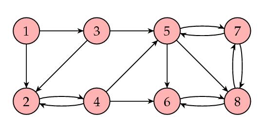
In this case, the matrix S is
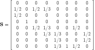 |
with stationary vector
| 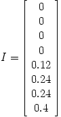 |
Notice that the PageRanks assigned to the first four web pages are zero. However, this doesn't feel right: each of these pages has links coming to them from other pages. Clearly, somebody likes these pages! Generally speaking, we want the importance rankings of all pages to be positive. The problem with this example is that it contains a smaller web within it, shown in the blue box below.
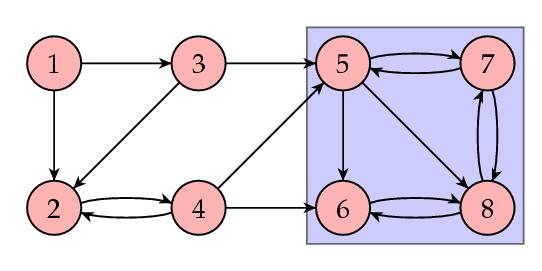
Links come into this box, but none go out. Just as in the example of the dangling node we discussed above, these pages form an "importance sink" that drains the importance out of the other four pages. This happens when the matrix S is reducible; that is, S can be written in block form as
![\[ S=\left[\begin{array}{cc} * & 0 \\ * & * \end{array}\right]. \]](http://www.ams.org/featurecolumn/images/december2006/index_39.gif)
Indeed, if the matrix S is irreducible, we can guarantee that there is a stationary vector with all positive entries.
A web is called strongly connected if, given any two pages, there is a way to follow links from the first page to the second. Clearly, our most recent example is not strongly connected. However, strongly connected webs provide irreducible matrices S.
To summarize, the matrix S is stochastic, which implies that it has a stationary vector. However, we need S to also be (a) primitive so that  and (b) irreducible so that the stationary vector has all positive entries.
A final modification
To find a new matrix that is both primitive and irreducible, we will modify the way our random surfer moves through the web. As it stands now, the movement of our random surfer is determined by S: either he will follow one of the links on his current page or, if at a page with no links, randomly choose any other page to move to. To make our modification, we will first choose a parameter  between 0 and 1. Now suppose that our random surfer moves in a slightly different way. With probability , he is guided by S. With probability  , he chooses the next page at random.
If we denote by 1 the  matrix whose entries are all one, we obtain the Google matrix:
![\[ {\bf G}=\alpha{\bf S}+ (1-\alpha)\frac{1}{n}{\bf 1} \]](http://www.ams.org/featurecolumn/images/december2006/index_44.gif)
Notice now that G is stochastic as it is a combination of stochastic matrices. Furthermore, all the entries of G are positive, which implies that Gis both primitive and irreducible. Therefore, G has a unique stationary vector I that may be found using the power method.
The role of the parameter is an important one. Notice that if  , then G = S. This means that we are working with the original hyperlink structure of the web. However, if  , then  . In other words, the web we are considering has a link between any two pages and we have lost the original hyperlink structure of the web. Clearly, we would like to take close to 1 so that we hyperlink structure of the web is weighted heavily into the computation.
However, there is another consideration. Remember that the rate of convergence of the power method is governed by the magnitude of the second eigenvalue  . For the Google matrix, it has been proven that the magnitude of the second eigenvalue  . This means that when is close to 1 the convergence of the power method will be very slow. As a compromise between these two competing interests, Serbey Brin and Larry Page, the creators of PageRank, chose  .
Computing I
What we've described so far looks like a good theory, but remember that we need to apply it to  matrices where n is about 25 billion! In fact, the power method is especially well-suited to this situation.
Remember that the stochastic matrix S may be written as
![\[ {\bf S}={\bf H} + {\bf A} \]](http://www.ams.org/featurecolumn/images/december2006/index_52.gif)
and therefore the Google matrix has the form
![\[ {\bf G}=\alpha{\bf H} + \alpha{\bf A} + \frac{1-\alpha}{n}{\bf 1} \]](http://www.ams.org/featurecolumn/images/december2006/index_53.gif)
Therefore,
![\[ {\bf G}I^k=\alpha{\bf H}I^k + \alpha{\bf A}I^k + \frac{1-\alpha}{n}{\bf 1}I^k \]](http://www.ams.org/featurecolumn/images/december2006/index_54.gif)
Now recall that most of the entries in H are zero; on average, only ten entries per column are nonzero. Therefore, evaluating HI k requires only ten nonzero terms for each entry in the resulting vector. Also, the rows of A are all identical as are the rows of 1. Therefore, evaluatingAI k and 1I k amounts to adding the current importance rankings of the dangling nodes or of all web pages. This only needs to be done once.
With the value of chosen to be near 0.85, Brin and Page report that 50 - 100 iterations are required to obtain a sufficiently good approximation to I. The calculation is reported to take a few days to complete.
Of course, the web is continually changing. First, the content of web pages, especially for news organizations, may change frequently. In addition, the underlying hyperlink structure of the web changes as pages are added or removed and links are added or removed. It is rumored that Google recomputes the PageRank vector I roughly every month. Since the PageRank of pages can be observed to fluctuate considerably during this time, it is known to some as the Google Dance. (In 2002, Google held a Google Dance!)
Summary
Brin and Page introduced Google in 1998, a time when the pace at which the web was growing began to outstrip the ability of current search engines to yield useable results. At that time, most search engines had been developed by businesses who were not interested in publishing the details of how their products worked. In developing Google, Brin and Page wanted to "push more development and understanding into the academic realm." That is, they hoped, first of all, to improve the design of search engines by moving it into a more open, academic environment. In addition, they felt that the usage statistics for their search engine would provide an interesting data set for research. It appears that the federal government, which recently tried to gain some of Google's statistics, feels the same way.
There are other algorithms that use the hyperlink structure of the web to rank the importance of web pages. One notable example is the HITS algorithm, produced by Jon Kleinberg, which forms the basis of the Teoma search engine. In fact, it is interesting to compare the results of searches sent to different search engines as a way to understand why some complain of a Googleopoly.
References
- Michael Berry, Murray Browne, Understanding Search Engines: Mathematical Modeling and Text Retrieval. Second Edition, SIAM, Philadelphia. 2005.
- Sergey Brin, Lawrence Page, The antaomy of a large-scale hypertextual Web search engine, Computer Networks and ISDN Systems,33: 107-17, 1998. Also available online at http://infolab.stanford.edu/pub/papers/google.pdf
- Kurt Bryan, Tanya Leise, The $25,000,000,000 eigenvector. The linear algebra behind Google. SIAM Review, 48 (3), 569-81. 2006. Also avaiable at http://www.rose-hulman.edu/~bryan/google.html
- Google Corporate Information: Technology.
- Taher Haveliwala, Sepandar Kamvar, The second eigenvalue of the Google matrix.
- Amy Langville, Carl Meyer, Google's PageRank and Beyond: The Science of Search Engine Rankings. Princeton University Press, 2006.
This is an informative, accessible book, written in an engaging style. Besides providing the relevant mathematical background and details of PageRank and its implementation (as well as Kleinberg's HITS algorithm), this book contains many interesting "Asides" that give trivia illuminating the context of search engine design.
NOTE: Those who can access JSTOR can find some of the papers mentioned above there. For those with access, the American Mathematical Society's MathSciNet can be used to get additional bibliographic information and reviews of some these materials. Some of the items above can be accessed via the ACM Portal, which also provides bibliographic services.
| 

 Markov Chains
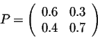
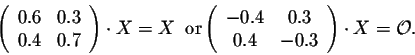
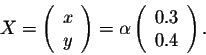
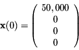
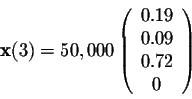
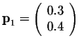 is a steady state vector of the matrix above. So if the populations of the city and the suburbs are given by the vector
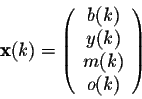
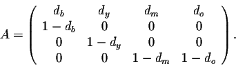
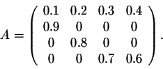
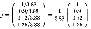
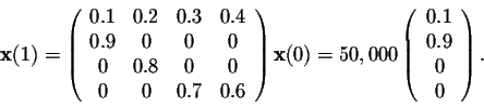
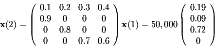
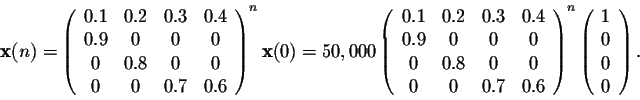
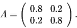


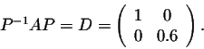

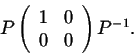
 , then we have
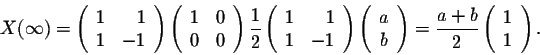


 Translate